T Test

** The T-test**

Additional Tutorials and Resources for t-tests

t-tests

1: Load packages

library(tidyverse)
library(see)
library(car)
library(patchwork)
library(ggsci)
library(ggridges)
library(performance)
library(car) #contains some statistical tests we need to assess assumptions

A note on statistics and experimental design

Statistics is a complex field with a long history. We could spend an entire course or even an entire career focusing on the intricate details of statistical decisions and ideas. We’ve already spent some time on this! I want you to have the statistical grounding necessary to plan your experiments and analyze your data. For biologists, statistics are a tool we can leverage to perform the best possible experiments and test our hypotheses. The T-test is the start of our stats journey. It’s a simple test and one that you may not use often, but the theory behind it sets the stage for what is to come!

T-test theory

The t-test (or students’ t-test) is a basic statistical test used to assess whether or not the means of two groups are different from one another. In this test, the null hypothesis is that the two means are equal (or that there is no difference between the two means).

A t-test should only be used if the following assumptions are met:
1.) the two distributions whose means we are comparing must be normally distributed
2.) The variances of the two groups must be equal

Generate example data

iris2<-iris %>%
  filter(Species != 'setosa') %>%
  droplevels() #removes the empty levels so when we check levels below we only get the ones that are still in the data!

#check levels to make sure we only have 2 species!
head(iris2)

  Sepal.Length Sepal.Width Petal.Length Petal.Width    Species
1          7.0         3.2          4.7         1.4 versicolor
2          6.4         3.2          4.5         1.5 versicolor
3          6.9         3.1          4.9         1.5 versicolor
4          5.5         2.3          4.0         1.3 versicolor
5          6.5         2.8          4.6         1.5 versicolor
6          5.7         2.8          4.5         1.3 versicolor

levels(iris2$Species)

[1] "versicolor" "virginica" 

We will use these data for our examples today. T-test requires only 2 groups/populations. We will assess the alternative hypothesis that one of our numerical variables (sepal length, sepal width, petal length, or petal width) differs by species.

But first, we must test our assumptions

Assumption 1.) Assessing normality

Method 1: the Shapiro-Wilk Test If p < 0.05 then the distribution is significantly different from normal.

Step 1: we need to create separate data frames for each species to assess normality of each variable by species!

versi<-iris2 %>%
  filter(Species=='versicolor') %>%
  droplevels()

virg<-iris2 %>%
  filter(Species=='virginica') %>%
  droplevels()

Step 2: We can run our shapiro-wilk tests on each variable if we’d like

shapiro.test(versi$Petal.Length) #this is normally distributed

    Shapiro-Wilk normality test

data:  versi$Petal.Length
W = 0.966, p-value = 0.1585

shapiro.test(versi$Petal.Width) # this is not

    Shapiro-Wilk normality test

data:  versi$Petal.Width
W = 0.94763, p-value = 0.02728

shapiro.test(versi$Sepal.Length) #normal

    Shapiro-Wilk normality test

data:  versi$Sepal.Length
W = 0.97784, p-value = 0.4647

shapiro.test(versi$Sepal.Width) #normal

    Shapiro-Wilk normality test

data:  versi$Sepal.Width
W = 0.97413, p-value = 0.338

shapiro.test(virg$Petal.Length) #normal

    Shapiro-Wilk normality test

data:  virg$Petal.Length
W = 0.96219, p-value = 0.1098

shapiro.test(virg$Petal.Width) #normal

    Shapiro-Wilk normality test

data:  virg$Petal.Width
W = 0.95977, p-value = 0.08695

shapiro.test(virg$Sepal.Length) #normal

    Shapiro-Wilk normality test

data:  virg$Sepal.Length
W = 0.97118, p-value = 0.2583

shapiro.test(virg$Sepal.Width) #normal

    Shapiro-Wilk normality test

data:  virg$Sepal.Width
W = 0.96739, p-value = 0.1809

Method 2: Visualization

Explore the following visualizations. Do you see clear evidence of normality?

a1<-ggplot(data=iris2, aes(Petal.Length, fill=Species))+
  geom_histogram(binwidth = 0.3)+ 
  facet_wrap(~Species)+
  theme_classic()+
  scale_fill_aaas()

a2<-ggplot(data=iris2, aes(x=Petal.Length, y=Species, fill=Species))+
  geom_density_ridges()+ #makes a smooth density curve instead of a histogram!
  theme_classic()+
  scale_fill_aaas()

a1/a2 #compare the visualizations (they are of the same data)- do we see normality here?

Picking joint bandwidth of 0.206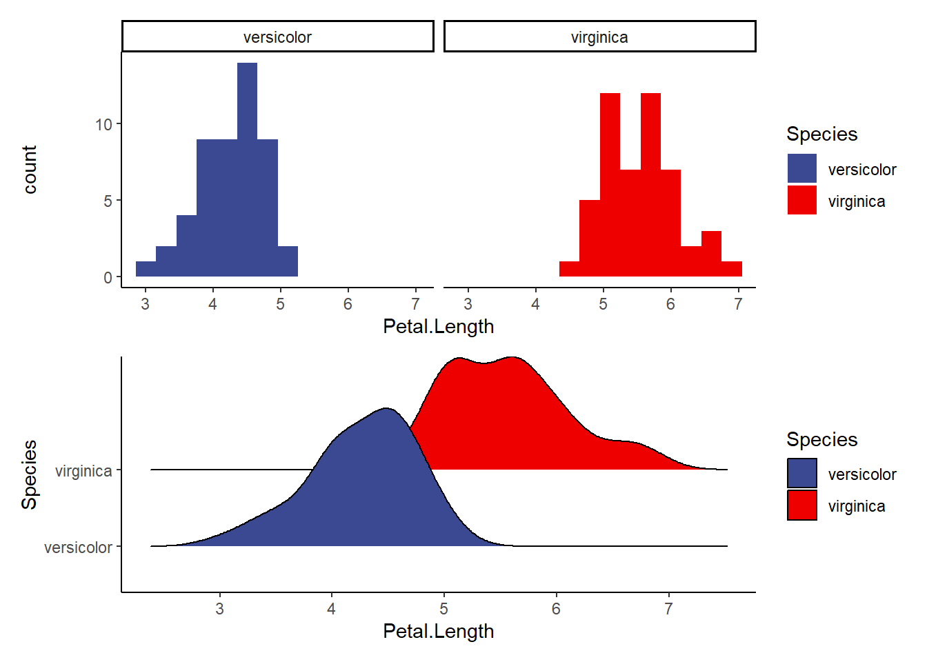

b1<-ggplot(data=iris2, aes(Petal.Width, fill=Species))+
  geom_histogram(binwidth = 0.3)+ 
  facet_wrap(~Species)+
  theme_classic()+
  scale_fill_aaas()

b2<-ggplot(data=iris2, aes(x=Petal.Width, y=Species, fill=Species))+
  geom_density_ridges()+ #makes a smooth density curve instead of a histogram!
  theme_classic()+
  scale_fill_aaas()

b1/b2 #compare the visualizations (they are of the same data)- do we see normality here?

Picking joint bandwidth of 0.0972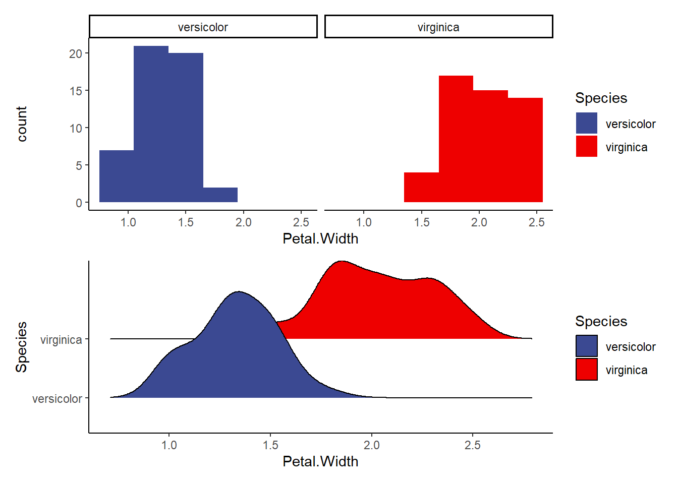

c1<-ggplot(data=iris2, aes(Sepal.Width, fill=Species))+
  geom_histogram(binwidth = 0.3)+ 
  facet_wrap(~Species)+
  theme_classic()+
  scale_fill_aaas()

c2<-ggplot(data=iris2, aes(x=Sepal.Width, y=Species, fill=Species))+
  geom_density_ridges()+ #makes a smooth density curve instead of a histogram!
  theme_classic()+
  scale_fill_aaas()

c1/c2 #compare the visualizations (they are of the same data)- do we see normality here?

Picking joint bandwidth of 0.122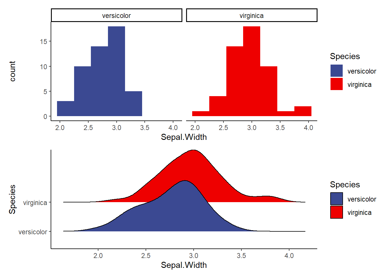

d1<-ggplot(data=iris2, aes(Sepal.Length, fill=Species))+
  geom_histogram(binwidth = 0.3)+ 
  facet_wrap(~Species)+
  theme_classic()+
  scale_fill_aaas()

d2<-ggplot(data=iris2, aes(x=Sepal.Length, y=Species, fill=Species))+
  geom_density_ridges()+ #makes a smooth density curve instead of a histogram!
  theme_classic()+
  scale_fill_aaas()

d1/d2 #compare the visualizations (they are of the same data)- do we see normality here?

Picking joint bandwidth of 0.21

Assumption 2.) Assessing equal variance

AKA homogeneity of variance

Methods 1: F-test We will use the F-Test to compare the variance of two populations. This can only be used with 2 populations and is thus only useful when we run a t-test.

H0 for an F-test is: The variances of the two groups are equal.
Ha: The variances are different
p<0.05 allows us to reject the null (H0) and suggests that the variances are different

note: The F-test assumes our data are already normal! You should not run it on non-normal data

#we use var.test to run an F-test
f1<- var.test(Petal.Length ~ Species, data=iris2)
f1 # p>0.05, so we fail to reject H0 (the variances are likely equal)

    F test to compare two variances

data:  Petal.Length by Species
F = 0.72497, num df = 49, denom df = 49, p-value = 0.2637
alternative hypothesis: true ratio of variances is not equal to 1
95 percent confidence interval:
 0.411402 1.277530
sample estimates:
ratio of variances 
         0.7249678 

f2<- var.test(Petal.Width ~ Species, data=iris2)
f2 # p<0.05, so we reject H0 (variances are likely different)

    F test to compare two variances

data:  Petal.Width by Species
F = 0.51842, num df = 49, denom df = 49, p-value = 0.02335
alternative hypothesis: true ratio of variances is not equal to 1
95 percent confidence interval:
 0.2941935 0.9135614
sample estimates:
ratio of variances 
         0.5184243 

f3<- var.test(Sepal.Length ~ Species, data=iris2)
f3 # p>0.05, so we fail to reject H0 (the variances are likely equal)

    F test to compare two variances

data:  Sepal.Length by Species
F = 0.65893, num df = 49, denom df = 49, p-value = 0.1478
alternative hypothesis: true ratio of variances is not equal to 1
95 percent confidence interval:
 0.3739257 1.1611546
sample estimates:
ratio of variances 
         0.6589276 

f4<- var.test(Sepal.Width ~ Species, data=iris2)
f4 # p>0.05, so we fail to reject H0 (the variances are likely equal)

    F test to compare two variances

data:  Sepal.Width by Species
F = 0.94678, num df = 49, denom df = 49, p-value = 0.849
alternative hypothesis: true ratio of variances is not equal to 1
95 percent confidence interval:
 0.5372773 1.6684117
sample estimates:
ratio of variances 
         0.9467839 

Method 2: Levene Test
A more flexible test of homogeneity of variance is the Levene Test. It can be used to compare the variance of many populations (not just 2) and is more flexible than the F-test, so it can be used even if the normality assumption is violated.
this is the most commonly used test for homogeneity of variance
leveneTest() is in the car package in R!

N0: Variances of all populations are equal
p<0.05 allows us to reject H0

l1<- leveneTest(Petal.Length ~ Species, data=iris2)
l1 # p>0.05, so we fail to reject H0 (the variances are likely equal)

Levene's Test for Homogeneity of Variance (center = median)
      Df F value Pr(>F)
group  1  1.0674 0.3041
      98               

l2<- leveneTest(Petal.Width ~ Species, data=iris2)
l2 # p<0.05, so we reject H0 (variances are likely different)

Levene's Test for Homogeneity of Variance (center = median)
      Df F value  Pr(>F)  
group  1  6.5455 0.01205 *
      98                  
---
Signif. codes:  0 '***' 0.001 '**' 0.01 '*' 0.05 '.' 0.1 ' ' 1

l3<- leveneTest(Sepal.Length ~ Species, data=iris2)
l3 # p>0.05, so we fail to reject H0 (the variances are likely equal)

Levene's Test for Homogeneity of Variance (center = median)
      Df F value Pr(>F)
group  1  1.0245 0.3139
      98               

l4<- leveneTest(Sepal.Width ~ Species, data=iris2)
l4 # p>0.05, so we fail to reject H0 (the variances are likely equal)

Levene's Test for Homogeneity of Variance (center = median)
      Df F value Pr(>F)
group  1  0.0873 0.7683
      98               

Method 3: Visualization
Since p-values are more like guidelines, we also want to visualize our data to assess homogeneity of variance. We can do that in several ways. You might already have some ideas about this! In general, it seems smart to display the raw data as points and as boxplots. Let’s start there!

v1.1<-ggplot(data=iris2, aes(x=Species, y=Petal.Length, color=Species))+
  geom_point()+
  theme_classic()+
  scale_color_aaas()

v1.2<-ggplot(data=iris2, aes(x=Species, y=Petal.Length, color=Species))+
  geom_boxplot()+
  theme_classic()+
  scale_color_aaas()

v1.1+v1.2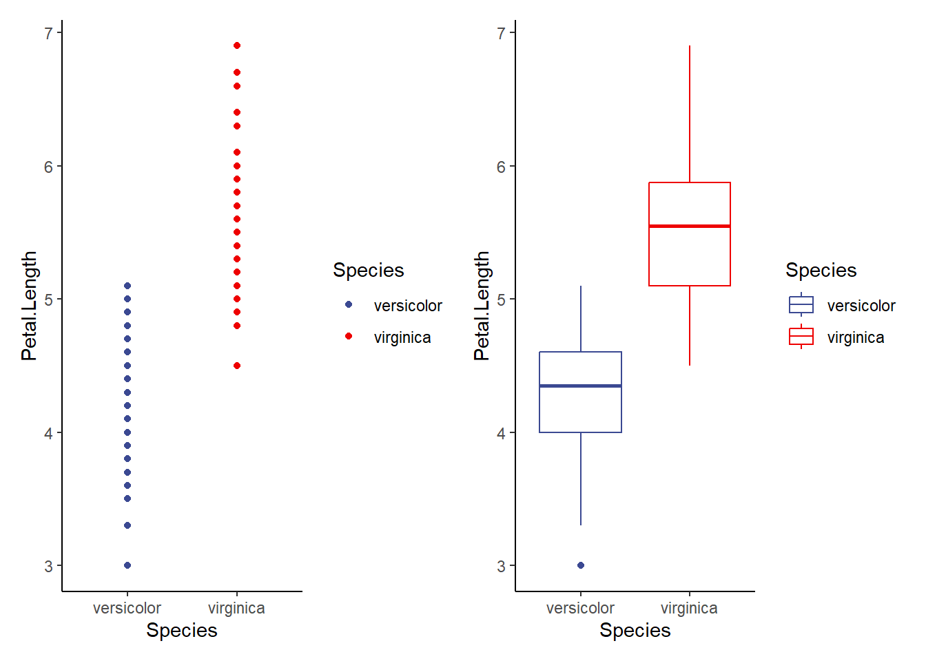

v2.1<-ggplot(data=iris2, aes(x=Species, y=Petal.Width, color=Species))+
  geom_point()+
  theme_classic()+
  scale_color_aaas()

v2.2<-ggplot(data=iris2, aes(x=Species, y=Petal.Width, color=Species))+
  geom_boxplot()+
  theme_classic()+
  scale_color_aaas()

v2.1+v2.2

v3.1<-ggplot(data=iris2, aes(x=Species, y=Sepal.Width, color=Species))+
  geom_point()+
  theme_classic()+
  scale_color_aaas()

v3.2<-ggplot(data=iris2, aes(x=Species, y=Sepal.Width, color=Species))+
  geom_boxplot()+
  theme_classic()+
  scale_color_aaas()

v3.1+v3.2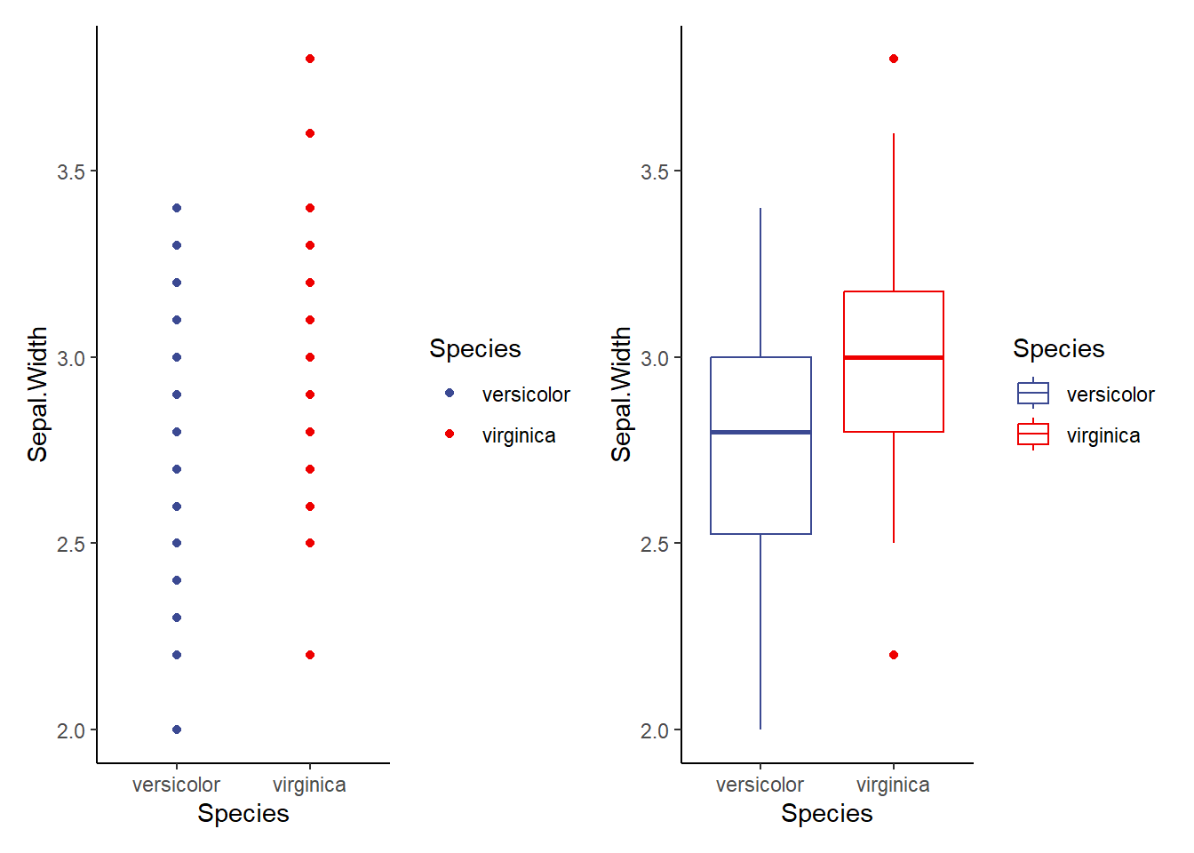

v4.1<-ggplot(data=iris2, aes(x=Species, y=Sepal.Length, color=Species))+
  geom_point()+
  theme_classic()+
  scale_color_aaas()

v4.2<-ggplot(data=iris2, aes(x=Species, y=Sepal.Length, color=Species))+
  geom_boxplot()+
  theme_classic()+
  scale_color_aaas()

v4.1+v4.2

When can we ignore assumptions?

We can if our sample sizes are large. If n is small, we should not ignore this assumption. There are alternatives to dealing with normality that we can discuss in the ANOVA section (such as transforming the data)

For more info on that

We can also ignore the equal variance requirement if we use the Welch t-test (default in R)

A basic T-test in R

Finally, let’s do some T-tests!

H0: No difference between the means of the 2 populations p<0.05 allows us to reject this H0 (indicating a likely difference)

Step 1: Calculate means and error and plot!

meaniris<-iris2 %>%
  group_by(Species) %>%
  dplyr::summarise(meanpl=mean(Petal.Length), sdpl=sd(Petal.Length), n=n(), sepl=sdpl/sqrt(n), meanpw=mean(Petal.Width), sdpw=sd(Petal.Width), n=n(), sepw=sdpw/sqrt(n), meansl=mean(Sepal.Length), sdsl=sd(Sepal.Length), n=n(), sesl=sdpl/sqrt(n), meansw=mean(Sepal.Width), sdsw=sd(Sepal.Width), n=n(), sesw=sdsw/sqrt(n))

meaniris

# A tibble: 2 × 14
  Species    meanpl  sdpl     n   sepl meanpw  sdpw   sepw meansl  sdsl   sesl
  <fct>       <dbl> <dbl> <int>  <dbl>  <dbl> <dbl>  <dbl>  <dbl> <dbl>  <dbl>
1 versicolor   4.26 0.470    50 0.0665   1.33 0.198 0.0280   5.94 0.516 0.0665
2 virginica    5.55 0.552    50 0.0780   2.03 0.275 0.0388   6.59 0.636 0.0780
# ℹ 3 more variables: meansw <dbl>, sdsw <dbl>, sesw <dbl>

p1<-ggplot(meaniris, aes(x=Species, y=meanpl, color=Species))+
  geom_point()+
  geom_errorbar(aes(x=Species, ymin=meanpl-sepl, ymax=meanpl+sepl), width=0.2)+
  scale_color_aaas()+
  theme_classic()+
  labs(title='Petal Length')

p2<-ggplot(meaniris, aes(x=Species, y=meanpw, color=Species))+
  geom_point()+
  geom_errorbar(aes(x=Species, ymin=meanpw-sepw, ymax=meanpw+sepw), width=0.2)+
  scale_color_aaas()+
  theme_classic()+
  labs(title='Petal Width')

p3<-ggplot(meaniris, aes(x=Species, y=meansl, color=Species))+
  geom_point()+
  geom_errorbar(aes(x=Species, ymin=meansl-sesl, ymax=meansl+sesl), width=0.2)+
  scale_color_aaas()+
  theme_classic()+
  labs(title='Sepal Length')

p4<-ggplot(meaniris, aes(x=Species, y=meansw, color=Species))+
  geom_point()+
  geom_errorbar(aes(x=Species, ymin=meansw-sesw, ymax=meansw+sesw), width=0.2)+
  scale_color_aaas()+
  theme_classic()+
  labs(title='Sepal Width')

(p1+p2)/(p3+p4)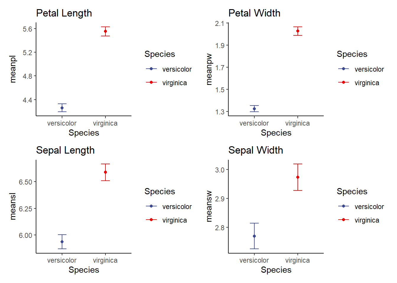

Does Petal Length differ by species?

t1<-t.test(data=iris2, Petal.Length~Species, alternative='two.sided', var.equal=FALSE) #two.sided and var.equal= FALSE are default, so we don't have to list them. BUt, we can also change them (as I will show later)

t1 #p<0.05 suggests that there is a significant difference in petal length between species

    Welch Two Sample t-test

data:  Petal.Length by Species
t = -12.604, df = 95.57, p-value < 2.2e-16
alternative hypothesis: true difference in means between group versicolor and group virginica is not equal to 0
95 percent confidence interval:
 -1.49549 -1.08851
sample estimates:
mean in group versicolor  mean in group virginica 
                   4.260                    5.552 

Our p<0.05 suggests that there is a significant effect of species on petal length (petal length differs by species). BUT, do we get a clear explanation of which group is higher or lower? Look at the Welch T-test output and you can see the means! You can also use the graph we made to visualize this!

Does Petal Width differ by species?

t2<-t.test(data=iris2, Petal.Width~Species, alternative='two.sided', var.equal=FALSE) #two.sided and var.equal= FALSE are default, so we don't have to list them. BUt, we can also change them (as I will show later)

t2

    Welch Two Sample t-test

data:  Petal.Width by Species
t = -14.625, df = 89.043, p-value < 2.2e-16
alternative hypothesis: true difference in means between group versicolor and group virginica is not equal to 0
95 percent confidence interval:
 -0.7951002 -0.6048998
sample estimates:
mean in group versicolor  mean in group virginica 
                   1.326                    2.026 

Does Sepal Width differ between species?

t3<-t.test(data=iris2, Sepal.Width~Species, alternative='two.sided', var.equal=FALSE) #two.sided and var.equal= FALSE are default, so we don't have to list them. BUt, we can also change them (as I will show later)

t3

    Welch Two Sample t-test

data:  Sepal.Width by Species
t = -3.2058, df = 97.927, p-value = 0.001819
alternative hypothesis: true difference in means between group versicolor and group virginica is not equal to 0
95 percent confidence interval:
 -0.33028364 -0.07771636
sample estimates:
mean in group versicolor  mean in group virginica 
                   2.770                    2.974 

Does Sepal Length differ between species?

t4<-t.test(data=iris2, Sepal.Length~Species, alternative='two.sided', var.equal=FALSE) #two.sided and var.equal= FALSE are default, so we don't have to list them. BUt, we can also change them (as I will show later)

t4

    Welch Two Sample t-test

data:  Sepal.Length by Species
t = -5.6292, df = 94.025, p-value = 1.866e-07
alternative hypothesis: true difference in means between group versicolor and group virginica is not equal to 0
95 percent confidence interval:
 -0.8819731 -0.4220269
sample estimates:
mean in group versicolor  mean in group virginica 
                   5.936                    6.588 

SO, when is a t-test actually useful and when isn’t it? We use a T-test ONLY when we want to compare two means / two populations. If we have more than 2 groups, a T-test is not appropriate! Instead, we need to use an analysis of variance (ANOVA) or possibly something more complex!