getwd()[1] "E:/Google Drive/Teaching/Bates College/ENV 282 - Research Design in Env Sci/ENVR282_website"IN THIS TUTORIAL YOU WILL LEARN:
1.) How to access and/or install R and RStudio
2.) How to navigate RStudio
3.) How to set and change the working directory
4.) How to setup an RStudio Project
5.) How to make a quarto doc
6.) Some R basics
Books and workshops for learning tidyverse
A nice step by step walkthough of Tidyverse functions
Want to TRY some stuff on your own? Use the RStudio.cloud primers
The best way to learn is to GOOGLE IT and try stuff
In this course we will learn how to program in R (a coding language) using RStudio (a coding environment). RStudio makes using R easier and more user friendly!
We will also learn how to make pdf and html output files that include code and outputs (tables and graphs).
These are handy tools for reporting data and even for writing papers! We will use Quarto to do this (a new tool from the folks who designed RStudio).
Your lab reports will all be built using Quarto.
You have options:
1. Install R and RStudio on your device(s) and use it locally
2. Sign up for a posit cloud account here: https://posit.cloud/plans/free. Posit Cloud is a way to access RStudio online without downloading and installing anything.
To install R, we will use this link: install R
1.) Choose the operating system you use (macosx or windows)
2.) Click the blue .pkg link that aligns with your computer and operating system (ask questions if needed)
3.) Follow instructions
1.) Click this link and follow instructions
2.) OPEN RStudio (not R). Click on the logo that is a white R inside a blue circle (RStudio). We never need to open R, we can use RStudio.
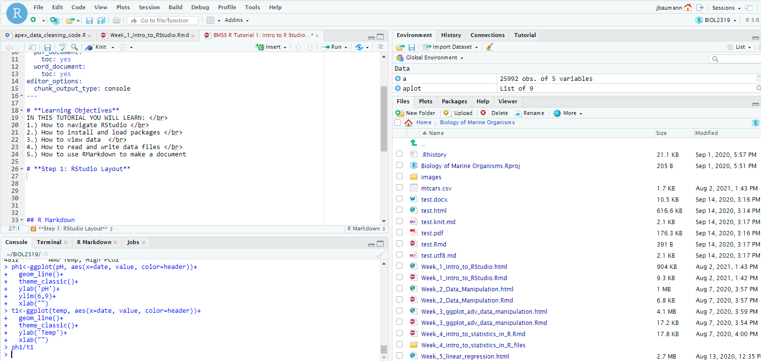
Where you will write your script(s). This is where we should be writing our code! It can be run, commented, and saved here.
Here you can run single lines of code and/or see error messages, warnings, and other outputs. Code should not be written here unless it is simple / for testing! Anything worth keeping should go in the script at the top left!
Here you will be able to see the dataframes you have read into R or created (using the “Environment tab”). The other tabs are less useful for us at this stage, but feel free to explore them! Note: The Broom icon can be used to clear dataframes from your environment. You can minimize or maximize this and each other quadrant using the symbols at the top right of the quadrant (a collapsed page next to a full page)
This is the second most important quadrant (behind top left) and we can change the working directory here very easily. Here we can see the files in our present working directory (we will learn about that next!) We can also see any plots we make in the plots tab. VERY importantly, we can see the packages we have loaded or installed in the packages tab. This will be useful to you! You can also use this tab to search the internal Help dictionary, though I will note that the internet is often more helpful!
You can use the top bar in RStudio much like in any other program. I’ll let you explore that on your own. Notably, in the top right corner of the top bar you will see an ‘R’ in a blue box. This is where you can set the project you are working form. Using projects is great because it allows you an easy way to compartmentalize your code, data, figures, and working directory for a single project all in one place! We will get to this shortly.
1.) We can use the getwd() command!
getwd()[1] "E:/Google Drive/Teaching/Bates College/ENV 282 - Research Design in Env Sci/ENVR282_website"2.) We can also use the Bottom Right “Files” tab
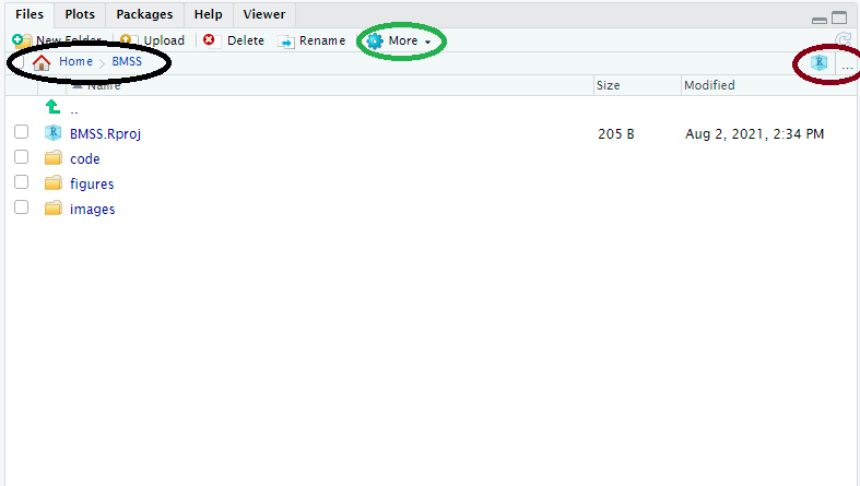
Here our working directory (and it’s file path) can be located in the black circle. We can manually change the working directory by using the ‘…’ in the brown circle to find any folder on our computer (or attached cloud folders), navigating to it, and then using the ‘More’ Cog in the green circle to “Set as working directory”
3.) An alternative approach to finding the working directory in the “Files” tab. Using the “More” cog, we can select “Go to working directory”
1.) Using the “Files” tab to set manually: a.) Using the ‘…’ in the ‘Files’ tab you can select any directory (folder) on your computer. You can also set a google drive, box, dropbox, or other shared folder as your working directory if you’d like (as long as you are syncing a folder between the cloud and your computer – ASK me if you have questions about this!) b.) Once you navigate to a directory you still need to SET IT as your working directory. You do this in the “More” cog– select “Set as working directory”
2.) Set working directory with code: We use the ‘setwd()’ function for this. Below is an example. You will need to replace the path details with your own!
setwd("C:/Users/Justin Baumann/Teaching/Bates College/ENV 282 - Research Design in Env Sci")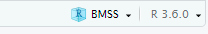
RStudio Projects are a great way to compartmentalize your coding work! You can store your code, outputs, input files, figures, etc all in one directory (with subdirectories). When you load your R Project, R will automatically load the last scripts you were working with on that project as well as the dataframes and items you have read in (your environment will be ready to go!). It will also navigate to the correct working directory automatically :) This will make your life easier!
To make an RStudio Project
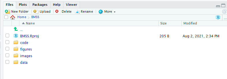
1.) Create a folder on your computer (or cloud storage) that will serve as the MAIN directory for your project. Within that folder I recommend you make subdirectories for all of your R related inputs and outputs. Maybe something like I have here:
2.) Once you have a MAIN directory folder created (whether you’ve made subdirectories or not) you can create a project! Set your main folder as your working directory. Next, navigate to the TOP RIGHT of your screen and select the down arrow next to the Big “R” in a blue box. NOW, select “New Project” –> Existing directory –> Name the project and hit done! At this point you will see a .Rproj file appear in your MAIN directory. This means you did it right :) This .Rproj file is how you save all of your project info. It autosaves and when you select your project (Again, TOP RIGHT of your screen, select the down arrow next to the R in the blue box and then select your project name) it will load up your scripts, environment, and set your working directory as the MAIN folder. You can navigate VERY easily from here :)
Quarto is a report building software that is integrated into RStudio. It replaces RMarkdown, if you have used that in the past, and is usable with python, julia, and R. Thus, learning it is a transferable skill. Quarto is designed to allow you to easily write documents that integrate text, hyperlinks, code, and images into a one neat file. This website, for example, is made entirely in Quarto! Quarto documents, or markdown documents as they are more generically known, are common in data science. these documents are great for courses, as you can do your programming, share your code, results, figures, stats, and explanations all in one document. Instead of the instructor downloading your code and running it line by line, we can see the results of the code you write just below the code itself! Super nice for assessing work. Plus, Quarto documents will not render unless the code is error free, so this is a nice way for students to check their own work.
Beyond course use, Quarto and markdown is excellent for creating professional looking data driven reports as well as online resources (like this website :) ). Learning Quarto is a great skill for anyone interested in programming, data, or the sciences! So, let’s learn how to use it!
click file -> new file -> Quarto document / Complete the pop up prompts and then wait for the document to load. / We want to replace the top bit (our YAML header, everything between the two lines that contains just — at the top) with the following (use your name and title!)
---
title: "Lab 1: Intro to R, RStudio, and Quarto"
author: "Justin Baumann"
format:
  html:
    toc: true
  pdf:
    toc: true
    number-sections: true
    colorlinks: true
    embed-resources: true

editor: visual
---
Unlike in a regular R script, using the ‘#’ at the start of a line will not comment that line out. Instead, you can type as you would normally in an R Markdown (Rmd) document. We can format our text in the following ways:
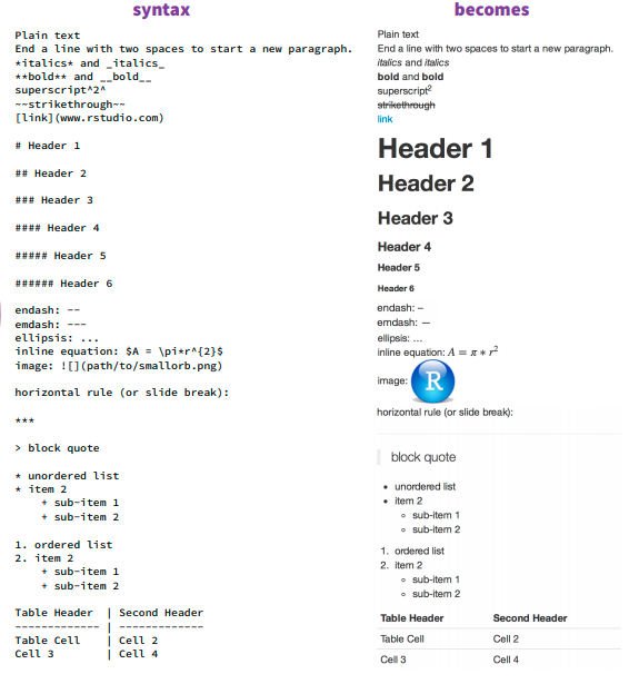
Bold: ‘’ on either end of a word, phrase, or line will make it bold! this is in bold** =’‘this is in bold’’ without the quotes around the **
Line breaks: DO you want text to be on different lines? Insert a ’’ at the end of a line to make a line break!
Since qmd documents are text based, we need to tell RStudio when we want to actually include code. To do this, we will insert a code chunk. To insert a code chunk:
1.) Use the keyboard shortcut ‘ctrl’+‘alt’+‘i’ (PC) or ‘cmd’+‘alt’+‘i’ (Mac) to insert a code chunk.
2.) Navigate to the top bar (of the top left quadrant of RStudio), find “+c” at the right of the bar to insert an R code chink.
Once you have a code chunk inserted you will notice that the background of the chunk is gray instead of your default background color (white or black if you are in dark mode)
#this is an example code chunk

# Using '#' at the start of a line indicates a comment, which is not runnable code!
To Visualize what your report will look like, click the ‘visual’ tab in the top bar (on the left). Note that if you do this, it CAN change your code–so be careful. You can also use the GUI to alter your report in the visual tab. This provides a nice alternative to the code based formatting options in the ‘source’ tab.
To actually render into an html or pdf document, you must click “Render”. You can use the arrow to the right of “Render” to choose render to html or render to pdf. I suggest using HTML most of the time but you can use pdf if you prefer. You will need to successfully Render your quarto document into an html or pdf report in order to turn in your labs!
Libraries are packages of functions (and sometimes data) that we use to execute tasks in R. Packages are what make R so versatile! We can do almost anything with R if we learn how to utilize the right packages.
If we do not have a package already installed (for example, if you have only just downloaded R/ RStudio), we will need to use install.packages(‘packagename’) to install each package that we need.
install.packages(tidyverse)OR - We can use the ‘Packages’ tab in the bottom right quadrant to install packages. Simply navigate to ‘Packages’, select ‘install packages’ and enter the package names you need (separate each package by commas).
In order for a package to work, we must first load it! We do this as with the code libary(packagename)
library(tidyverse) #for data manipulation
library(palmerpenguins) #for some fun data!
It is best practice to load all of the packages you will need at the top of your script
In this course we will be following a best practices guide that utilizes a library called ‘Tidyverse’ for data manipulation and analysis. Tidyverse contains many packages all in one, including the very functional ‘dplyr’ and ‘ggplot2’ packages. You will almost always use Tidyverse, so make sure to load it in :)
Note the ‘#’ with notes after them in the code chunk above. These are called comments. You can comment out any line of code in R by using a ‘#’. This is strongly recommended when you are programming. We will discuss more later!
R has integrated data sets that we can use to play around with code and learn.
examples: mtcars (a dataframe all about cars, this is available in R without loading a package), and iris (in the ‘vegan’ package, great for testing out ecology related functions and code)
Load a dataset R has some test datasets built into it. Let’s load one and look at it!
mtcars mpg cyl disp hp drat wt qsec vs am gear carb
Mazda RX4 21.0 6 160.0 110 3.90 2.620 16.46 0 1 4 4
Mazda RX4 Wag 21.0 6 160.0 110 3.90 2.875 17.02 0 1 4 4
Datsun 710 22.8 4 108.0 93 3.85 2.320 18.61 1 1 4 1
Hornet 4 Drive 21.4 6 258.0 110 3.08 3.215 19.44 1 0 3 1
Hornet Sportabout 18.7 8 360.0 175 3.15 3.440 17.02 0 0 3 2
Valiant 18.1 6 225.0 105 2.76 3.460 20.22 1 0 3 1
Duster 360 14.3 8 360.0 245 3.21 3.570 15.84 0 0 3 4
Merc 240D 24.4 4 146.7 62 3.69 3.190 20.00 1 0 4 2
Merc 230 22.8 4 140.8 95 3.92 3.150 22.90 1 0 4 2
Merc 280 19.2 6 167.6 123 3.92 3.440 18.30 1 0 4 4
Merc 280C 17.8 6 167.6 123 3.92 3.440 18.90 1 0 4 4
Merc 450SE 16.4 8 275.8 180 3.07 4.070 17.40 0 0 3 3
Merc 450SL 17.3 8 275.8 180 3.07 3.730 17.60 0 0 3 3
Merc 450SLC 15.2 8 275.8 180 3.07 3.780 18.00 0 0 3 3
Cadillac Fleetwood 10.4 8 472.0 205 2.93 5.250 17.98 0 0 3 4
Lincoln Continental 10.4 8 460.0 215 3.00 5.424 17.82 0 0 3 4
Chrysler Imperial 14.7 8 440.0 230 3.23 5.345 17.42 0 0 3 4
Fiat 128 32.4 4 78.7 66 4.08 2.200 19.47 1 1 4 1
Honda Civic 30.4 4 75.7 52 4.93 1.615 18.52 1 1 4 2
Toyota Corolla 33.9 4 71.1 65 4.22 1.835 19.90 1 1 4 1
Toyota Corona 21.5 4 120.1 97 3.70 2.465 20.01 1 0 3 1
Dodge Challenger 15.5 8 318.0 150 2.76 3.520 16.87 0 0 3 2
AMC Javelin 15.2 8 304.0 150 3.15 3.435 17.30 0 0 3 2
Camaro Z28 13.3 8 350.0 245 3.73 3.840 15.41 0 0 3 4
Pontiac Firebird 19.2 8 400.0 175 3.08 3.845 17.05 0 0 3 2
Fiat X1-9 27.3 4 79.0 66 4.08 1.935 18.90 1 1 4 1
Porsche 914-2 26.0 4 120.3 91 4.43 2.140 16.70 0 1 5 2
Lotus Europa 30.4 4 95.1 113 3.77 1.513 16.90 1 1 5 2
Ford Pantera L 15.8 8 351.0 264 4.22 3.170 14.50 0 1 5 4
Ferrari Dino 19.7 6 145.0 175 3.62 2.770 15.50 0 1 5 6
Maserati Bora 15.0 8 301.0 335 3.54 3.570 14.60 0 1 5 8
Volvo 142E 21.4 4 121.0 109 4.11 2.780 18.60 1 1 4 2Using head() and tail() Now let’s look at the data frame (df) using head() and tail()
These tell us the column names, and let us see the top or bottom 6 rows of data.
head(mtcars) mpg cyl disp hp drat wt qsec vs am gear carb
Mazda RX4 21.0 6 160 110 3.90 2.620 16.46 0 1 4 4
Mazda RX4 Wag 21.0 6 160 110 3.90 2.875 17.02 0 1 4 4
Datsun 710 22.8 4 108 93 3.85 2.320 18.61 1 1 4 1
Hornet 4 Drive 21.4 6 258 110 3.08 3.215 19.44 1 0 3 1
Hornet Sportabout 18.7 8 360 175 3.15 3.440 17.02 0 0 3 2
Valiant 18.1 6 225 105 2.76 3.460 20.22 1 0 3 1tail(mtcars) #tail shows the header and the last 6 rows mpg cyl disp hp drat wt qsec vs am gear carb
Porsche 914-2 26.0 4 120.3 91 4.43 2.140 16.7 0 1 5 2
Lotus Europa 30.4 4 95.1 113 3.77 1.513 16.9 1 1 5 2
Ford Pantera L 15.8 8 351.0 264 4.22 3.170 14.5 0 1 5 4
Ferrari Dino 19.7 6 145.0 175 3.62 2.770 15.5 0 1 5 6
Maserati Bora 15.0 8 301.0 335 3.54 3.570 14.6 0 1 5 8
Volvo 142E 21.4 4 121.0 109 4.11 2.780 18.6 1 1 4 2column attributes If we want to see the attributes of each column we can use the str() function
str(mtcars) #str shows attributes of each column'data.frame': 32 obs. of 11 variables:
$ mpg : num 21 21 22.8 21.4 18.7 18.1 14.3 24.4 22.8 19.2 ...
$ cyl : num 6 6 4 6 8 6 8 4 4 6 ...
$ disp: num 160 160 108 258 360 ...
$ hp : num 110 110 93 110 175 105 245 62 95 123 ...
$ drat: num 3.9 3.9 3.85 3.08 3.15 2.76 3.21 3.69 3.92 3.92 ...
$ wt : num 2.62 2.88 2.32 3.21 3.44 ...
$ qsec: num 16.5 17 18.6 19.4 17 ...
$ vs : num 0 0 1 1 0 1 0 1 1 1 ...
$ am : num 1 1 1 0 0 0 0 0 0 0 ...
$ gear: num 4 4 4 3 3 3 3 4 4 4 ...
$ carb: num 4 4 1 1 2 1 4 2 2 4 ...str() is very important because it allows you to see the type of data in each column. Types include: integer, numeric, factor, date, and more. If the data in a column are factors instead of numbers you may have an issue in your data (your spreadsheet)
Changing column attributes Importantly, you can change the type of the column. Here is an example
mtcars$mpg=as.factor(mtcars$mpg) # Makes mpg a factor instead of a number
str(mtcars)
'data.frame': 32 obs. of 11 variables:
$ mpg : Factor w/ 25 levels "10.4","13.3",..: 16 16 19 17 13 12 3 20 19 14 ...
$ cyl : num 6 6 4 6 8 6 8 4 4 6 ...
$ disp: num 160 160 108 258 360 ...
$ hp : num 110 110 93 110 175 105 245 62 95 123 ...
$ drat: num 3.9 3.9 3.85 3.08 3.15 2.76 3.21 3.69 3.92 3.92 ...
$ wt : num 2.62 2.88 2.32 3.21 3.44 ...
$ qsec: num 16.5 17 18.6 19.4 17 ...
$ vs : num 0 0 1 1 0 1 0 1 1 1 ...
$ am : num 1 1 1 0 0 0 0 0 0 0 ...
$ gear: num 4 4 4 3 3 3 3 4 4 4 ...
$ carb: num 4 4 1 1 2 1 4 2 2 4 ...mtcars$mpg=as.numeric(as.character(mtcars$mpg)) #Changes mpg back to a number
str(mtcars)'data.frame': 32 obs. of 11 variables:
$ mpg : num 21 21 22.8 21.4 18.7 18.1 14.3 24.4 22.8 19.2 ...
$ cyl : num 6 6 4 6 8 6 8 4 4 6 ...
$ disp: num 160 160 108 258 360 ...
$ hp : num 110 110 93 110 175 105 245 62 95 123 ...
$ drat: num 3.9 3.9 3.85 3.08 3.15 2.76 3.21 3.69 3.92 3.92 ...
$ wt : num 2.62 2.88 2.32 3.21 3.44 ...
$ qsec: num 16.5 17 18.6 19.4 17 ...
$ vs : num 0 0 1 1 0 1 0 1 1 1 ...
$ am : num 1 1 1 0 0 0 0 0 0 0 ...
$ gear: num 4 4 4 3 3 3 3 4 4 4 ...
$ carb: num 4 4 1 1 2 1 4 2 2 4 ...Summary statistics To see summary statistics on each column (mean, median, min, max, range), we can use summary()
summary(mtcars) #summarizes each column mpg cyl disp hp
Min. :10.40 Min. :4.000 Min. : 71.1 Min. : 52.0
1st Qu.:15.43 1st Qu.:4.000 1st Qu.:120.8 1st Qu.: 96.5
Median :19.20 Median :6.000 Median :196.3 Median :123.0
Mean :20.09 Mean :6.188 Mean :230.7 Mean :146.7
3rd Qu.:22.80 3rd Qu.:8.000 3rd Qu.:326.0 3rd Qu.:180.0
Max. :33.90 Max. :8.000 Max. :472.0 Max. :335.0
drat wt qsec vs
Min. :2.760 Min. :1.513 Min. :14.50 Min. :0.0000
1st Qu.:3.080 1st Qu.:2.581 1st Qu.:16.89 1st Qu.:0.0000
Median :3.695 Median :3.325 Median :17.71 Median :0.0000
Mean :3.597 Mean :3.217 Mean :17.85 Mean :0.4375
3rd Qu.:3.920 3rd Qu.:3.610 3rd Qu.:18.90 3rd Qu.:1.0000
Max. :4.930 Max. :5.424 Max. :22.90 Max. :1.0000
am gear carb
Min. :0.0000 Min. :3.000 Min. :1.000
1st Qu.:0.0000 1st Qu.:3.000 1st Qu.:2.000
Median :0.0000 Median :4.000 Median :2.000
Mean :0.4062 Mean :3.688 Mean :2.812
3rd Qu.:1.0000 3rd Qu.:4.000 3rd Qu.:4.000
Max. :1.0000 Max. :5.000 Max. :8.000 Counting rows and columns To see the number of rows and columns we can use nrow() and ncol()
nrow(mtcars) #gives number of rows[1] 32ncol(mtcars) #gives number of columns[1] 11Naming dataframes Rename mtcars and view in Environment tab in Rstudio
a<-mtcars
a
mpg cyl disp hp drat wt qsec vs am gear carb
Mazda RX4 21.0 6 160.0 110 3.90 2.620 16.46 0 1 4 4
Mazda RX4 Wag 21.0 6 160.0 110 3.90 2.875 17.02 0 1 4 4
Datsun 710 22.8 4 108.0 93 3.85 2.320 18.61 1 1 4 1
Hornet 4 Drive 21.4 6 258.0 110 3.08 3.215 19.44 1 0 3 1
Hornet Sportabout 18.7 8 360.0 175 3.15 3.440 17.02 0 0 3 2
Valiant 18.1 6 225.0 105 2.76 3.460 20.22 1 0 3 1
Duster 360 14.3 8 360.0 245 3.21 3.570 15.84 0 0 3 4
Merc 240D 24.4 4 146.7 62 3.69 3.190 20.00 1 0 4 2
Merc 230 22.8 4 140.8 95 3.92 3.150 22.90 1 0 4 2
Merc 280 19.2 6 167.6 123 3.92 3.440 18.30 1 0 4 4
Merc 280C 17.8 6 167.6 123 3.92 3.440 18.90 1 0 4 4
Merc 450SE 16.4 8 275.8 180 3.07 4.070 17.40 0 0 3 3
Merc 450SL 17.3 8 275.8 180 3.07 3.730 17.60 0 0 3 3
Merc 450SLC 15.2 8 275.8 180 3.07 3.780 18.00 0 0 3 3
Cadillac Fleetwood 10.4 8 472.0 205 2.93 5.250 17.98 0 0 3 4
Lincoln Continental 10.4 8 460.0 215 3.00 5.424 17.82 0 0 3 4
Chrysler Imperial 14.7 8 440.0 230 3.23 5.345 17.42 0 0 3 4
Fiat 128 32.4 4 78.7 66 4.08 2.200 19.47 1 1 4 1
Honda Civic 30.4 4 75.7 52 4.93 1.615 18.52 1 1 4 2
Toyota Corolla 33.9 4 71.1 65 4.22 1.835 19.90 1 1 4 1
Toyota Corona 21.5 4 120.1 97 3.70 2.465 20.01 1 0 3 1
Dodge Challenger 15.5 8 318.0 150 2.76 3.520 16.87 0 0 3 2
AMC Javelin 15.2 8 304.0 150 3.15 3.435 17.30 0 0 3 2
Camaro Z28 13.3 8 350.0 245 3.73 3.840 15.41 0 0 3 4
Pontiac Firebird 19.2 8 400.0 175 3.08 3.845 17.05 0 0 3 2
Fiat X1-9 27.3 4 79.0 66 4.08 1.935 18.90 1 1 4 1
Porsche 914-2 26.0 4 120.3 91 4.43 2.140 16.70 0 1 5 2
Lotus Europa 30.4 4 95.1 113 3.77 1.513 16.90 1 1 5 2
Ford Pantera L 15.8 8 351.0 264 4.22 3.170 14.50 0 1 5 4
Ferrari Dino 19.7 6 145.0 175 3.62 2.770 15.50 0 1 5 6
Maserati Bora 15.0 8 301.0 335 3.54 3.570 14.60 0 1 5 8
Volvo 142E 21.4 4 121.0 109 4.11 2.780 18.60 1 1 4 2head(a) mpg cyl disp hp drat wt qsec vs am gear carb
Mazda RX4 21.0 6 160 110 3.90 2.620 16.46 0 1 4 4
Mazda RX4 Wag 21.0 6 160 110 3.90 2.875 17.02 0 1 4 4
Datsun 710 22.8 4 108 93 3.85 2.320 18.61 1 1 4 1
Hornet 4 Drive 21.4 6 258 110 3.08 3.215 19.44 1 0 3 1
Hornet Sportabout 18.7 8 360 175 3.15 3.440 17.02 0 0 3 2
Valiant 18.1 6 225 105 2.76 3.460 20.22 1 0 3 1We use the write.csv function here. a= the name of the dataframe and the name we want to give the file goes after ‘file=’
The file name must be in quotes and must include an extension. Since we are using write.csv we MUST use .csv
write.csv(a, file='mtcars.csv')NOTE: if you have a .xls file make sure you convert to .csv. Ensure the file is clean and orderly (rows x columns). Only 1 excel tab can be in each .csv, so plan accordingly. Note that in order to read a file in to R from your computer (or cloud server), that file MUST be located within your working directory (or you must know and enter the file path).
IF your file is in your working directory, you can read it in like this:
b<-read.csv('mtcars.csv')
head(b)
X mpg cyl disp hp drat wt qsec vs am gear carb
1 Mazda RX4 21.0 6 160 110 3.90 2.620 16.46 0 1 4 4
2 Mazda RX4 Wag 21.0 6 160 110 3.90 2.875 17.02 0 1 4 4
3 Datsun 710 22.8 4 108 93 3.85 2.320 18.61 1 1 4 1
4 Hornet 4 Drive 21.4 6 258 110 3.08 3.215 19.44 1 0 3 1
5 Hornet Sportabout 18.7 8 360 175 3.15 3.440 17.02 0 0 3 2
6 Valiant 18.1 6 225 105 2.76 3.460 20.22 1 0 3 1You are welcome to use other functions to read in data (including read_csv or read.xls). Especially for beginners, I strongly encourage you to use .csv format. Other file formats can get complicated (often unnecessarily complicated). That said, R can also handle .txt, .xls, images, shapefiles (for spatial analysis or GIS style work), etc. It is very versatile! Feel free to explore :)
A note on read_csv -> I consider this to be the “best” option for reading in .csv files. It is a ‘smarter’ version of read.csv and can automatically figure out what kind of data (numeric, factor, date, etc) each column is. If you use read.csv, you have often have to manually change these options.
In some cases you may be using data you’ve found online. Perhaps you can download, save, and then read your file into R. Sometimes that is more work than we want to do. You can just call a file directly from it’s URL. Here is an example:
I have a dataframe on coral cover from Belize that I want to read in. It is located on my github coral cover data. Let’s read it directly into R! The URL you see above is NOT what we use in R. If you find a file on Github you want to locate the ‘raw’ version of the file. To do this:
1.) Click the link above (or find a data file on github)
2.) Navigate to the top right menu and look for the box that says “Raw” in it. You can click on that and open the raw file and then copy the URL. OR, you can click the box next to the “Raw” box to copy the link to the raw file. We use this link to read our data into R. This will work for any .csv you find on github. I like to get practice data from the TidyTuesday project on Github. You can find their data at the following link:
Tidy Tuesday Data
coralcover<- read_csv('https://raw.githubusercontent.com/jbaumann3/BIOL234_Biostats_MHC/main/coralcover.csv')Rows: 77 Columns: 6
── Column specification ────────────────────────────────────────────────────────
Delimiter: ","
chr (1): type
dbl (5): site, lat, transect, diver, cc_percent
ℹ Use `spec()` to retrieve the full column specification for this data.
ℹ Specify the column types or set `show_col_types = FALSE` to quiet this message.head(coralcover)# A tibble: 6 × 6
site type lat transect diver cc_percent
<dbl> <chr> <dbl> <dbl> <dbl> <dbl>
1 1 Back Reef 3 1 4 5.84
2 1 Back Reef 3 2 4 0.951
3 1 Back Reef 3 3 4 5.24
4 1 Back Reef 3 4 5 5.00
5 1 Back Reef 3 5 5 5.90
6 2 Patch Reef 3 1 4 5.28 1. Install R and Rstudio. Get Rstudio running on your computer and get familiar with the layout.
2. Make a folder (directory) on your computer for this course and then make an Rstudio project for this course that runs from that folder
3. Make a new quarto document, this is where you will do the lab assignment that you will turn in. Make a title and subject headers for each question. Copy the instructions and then add your work below. Make the question numbers bold. For numberr 1 (install Rstudio)- write me a short description of what you did (i.e.: “I installed R and Rstudio following this tutorial”), where “this” is a hyperlink to the tutorial you used (this lab, for example). For number 2: Set your folder for this class as your working directory. Navigate to it in the “files” tab on Rstudio. Take a screenshot and insert that screenshot as an image into your quarto doc.
4. Install the following packages: Tidyverse, lubridate, performance, palmerpenguins, patchwork, ggsci. Once installed, load them (using library()) in a code chunk in your quarto doc. remember that we generally want to load packages and any data at the top of our quarto doc, but for this assignment we will just do it in section 4.
5. Read in THESE data and take a look at the shape of the data using a.) head, b.) tail, c.) str(), d. summary (of a numeric column), and e.) count the number of rows and columns (using code!)
6. Change a numeric column to a factor.
7. Write your dataframe to file (save your dataframe as a .csv on your computer). It should save in your working directory. Next, read that file back in to R (This seems silly, but we are practicing!)
8. Render your file as a .html. Make sure you have “embed-resources: true” in your header. Please ask if you have questions! Once your file renders and saves it may open automatically (so you can check it). It also may not pop up automatically but you can find the .html in your working directory. If you get an error or the file doesn’t render, there is an error in your code somewhere (quarto docs ONLY render if there are no code errors).